Lab 7 - Midterm Review
1 Instructions
There are two parts: Part I (Causal Inference), Part II (Prediction). Use clear causal language and avoid causal claims for purely predictive models. Show work for any calculations.The data and required libraries are loaded with the chunk below.
data(Seatbelts, package = "datasets")
data(swiss, package = "datasets")
sb_df <- cbind.data.frame(as.data.frame(Seatbelts))
sb_df$year <- rep(1969:1984, each = 12)
sb_df$month <- rep(1:12, times = 16)

sw <- swiss
2 Part I — Causal Inference
Research Question: Did the introduction of the 1983 seat belt law in the UK reduce the number of monthly driver fatalities?
Dataset: Seatbelts
DriversKilled(monthly count)law(0 = before Jan 1983, 1 = after)monthkms(traffic volume)PetrolPriceVanKilled
- Research Design & Concepts
- What should we set as the outcome variable? What about the treatment variable?
The outcome variable is
DriversKilled. The treatment variable islaw.
- What is the unit of analysis?
The unit of analysis is the number of drivers killed per month.
- Why is this considered an observational rather than experimental study?
This study is observational since the researchers do not determine the treatment assignment.
- Average Causal Effect — Difference in Means Write R code to estimate
the difference in average DriversKilled before and after the law change.
You may use any method you know but
tapply()is recommended.
Example R code using
tapply()and without:
means <- tapply(sb_df$DriversKilled, sb_df$law, mean)
means[1]-means[2]
## 0
## 25.60895(mean(sb_df$DriversKilled[sb_df$law == 1]) - mean(sb_df$DriversKilled[sb_df$law == 0]))## [1] -25.60895- What quantity does this code estimate?
This code estimates the effect of the passage of the seatbelt law on the number of drivers killed.
- In 2–3 sentences, explain why this estimate might be biased.
The estimate may be biased because variables are omitted from the calculation of the effect. In the case of a binary predictor, difference in means estimator is equivalent to the coefficient on the binary predictor in a simple linear regression model (see below). Without controlling for confounding variables, the effect of these confounders would be incorporated into the model via the residuals (\(\varepsilon_i\)), meaning \(\mathbb{E}[\varepsilon_i] \neq 0\), which means that the effect \(\beta_1\) would be biased.
- Simple Linear Regression Interpretation Suppose you estimate:
m1 <- lm(DriversKilled ~ law, data = sb_df)
summary(m1)
##
## Call:
## lm(formula = DriversKilled ~ law, data = sb_df)
##
## Residuals:
## Min 1Q Median 3Q Max
## -46.870 -17.870 -5.565 14.130 72.130
##
## Coefficients:
## Estimate Std. Error t value Pr(>|t|)
## (Intercept) 125.870 1.849 68.082 < 2e-16 ***
## law -25.609 5.342 -4.794 3.29e-06 ***
## ---
## Signif. codes: 0 '***' 0.001 '**' 0.01 '*' 0.05 '.' 0.1 ' ' 1
##
## Residual standard error: 24.03 on 190 degrees of freedom
## Multiple R-squared: 0.1079, Adjusted R-squared: 0.1032
## F-statistic: 22.98 on 1 and 190 DF, p-value: 3.288e-06- Write the fitted regression equation.
The regression equation is:
\[ \texttt{DriversKilled}_i = \beta_0 + \beta_1\texttt{law}_i + \varepsilon_i \]
The fitted regression equation is:
\[ \texttt{DriversKilled}_i = 126 - 25.6\texttt{law}_i + \varepsilon_i \]
- Interpret the coefficients clearly in terms of this study. >
\(\beta_0\) is the contant term. The
value of the constant indicates to us the expected number of drivers
killed when
law\(=0\). In other words, the number of drivers killed when there is no seatbelt law.
\(\beta_1\) is the effect of
law. That is, whenlawincreases by \(1\), the number of drivers killed should increase by \(\beta_1\). In this case, with a binary predictorlaw, this means the effect of having a seatbelt law is that \(\beta_1\) more drivers are killed (note that \(\beta_1\) is likely negative, and therefore the effect should be a decrease in the number of drivers killed). c) Can this coefficient be interpreted as a causal effect? Why or why not? Which variable(s) might be a confounder?
The coefficient \(\beta_1\) cannot be interpreted as a causal effect because this effect may be confounded by other variables. For instance, there may have been more cars on the road after the passage of the law than before, which would indicate that \(\beta_1\) could be an underestimate of the effect of the seatbelt law.
- Confounding & Observational Design Name one specific variable that could confound the relationship between law and DriversKilled. Explain why it is a confounder.
See Above
- External Validity Would you expect this result to generalize to other countries? Would it generalize to the modern-day? Explain why or why not using correct causal language.
Other determinants of
DriversKilledmay have changed significantly from the period of observation of this study to now. For instance, the rate of drunk driving may have fallen dramatically. If more drunk driving causes less seatbelt usage and more drivers killed, then estimating the causal effect of the seatbelt law would require including drunk driving rates as a confounding variable.
3 Part II — Prediction
Research Question: Can socio-economic indicators predict fertility rates in Swiss provinces?
Dataset:
swiss
provinceFertilityEducationCatholicAgricultureInfant.Mortality
- Direction & Strength of Relationship Consider this scatter plot of Fertility vs Education.
plot(Fertility ~ Education, data = sw,
xlab = "Education (%) beyond primary (men)",
ylab = "Standardized Fertility"); abline(lm(Fertility ~ Education, data = sw))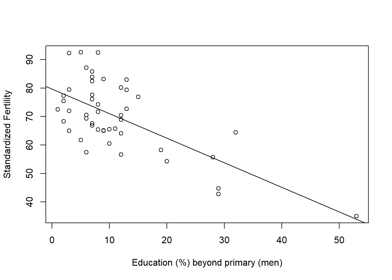
- Draw a line of best fit by hand. Is the relationship positive or negative?
Line of best fit shown in plot. The relationship is negative.
- Does it look strong or weak?
There seems to be a significant (good line fit) relationship, and the magnitude of the relationship looks strong (steep slope).
- Does this plot alone tell us if education causes lower fertility? Explain.
This plot alone does not tell us if education causes lower fertility as there are potential confounding variables not controlled for in the model. For instance, higher poverty in a region may cause higher fertility and lower education.
- Simple Regression with lm() Using
lm(), write a script to model the effect of education quality on fertility.
The code is shown below
g1 <- lm(Fertility ~ Education, data = sw)
summary(g1)
##
## Call:
## lm(formula = Fertility ~ Education, data = sw)
##
## Residuals:
## Min 1Q Median 3Q Max
## -17.036 -6.711 -1.011 9.526 19.689
##
## Coefficients:
## Estimate Std. Error t value Pr(>|t|)
## (Intercept) 79.6101 2.1041 37.836 < 2e-16 ***
## Education -0.8624 0.1448 -5.954 3.66e-07 ***
## ---
## Signif. codes: 0 '***' 0.001 '**' 0.01 '*' 0.05 '.' 0.1 ' ' 1
##
## Residual standard error: 9.446 on 45 degrees of freedom
## Multiple R-squared: 0.4406, Adjusted R-squared: 0.4282
## F-statistic: 35.45 on 1 and 45 DF, p-value: 3.659e-07Assume the output shows: \(\hat{\alpha} = 79.6\), \(\hat{\beta} = -0.86\).
- Write the fitted line.
The fitted line is:
\[ \texttt{Fertility}_i = 79.6 - 0.86 \texttt{Education}_i + \varepsilon_i \]
- Interpret \(\hat{\beta}\): If
Educationincreases by 1 unit (1 percentage point of men with post-primary education), how does predictedfertilitychange?
Each 1 unit increase in
Educationcorresponds to a 0.86 unit decrease infertility.
- Predict
fertilitywhenEducation= 15.
We can simply plug in
Education= 15 into the model above. In this caseFertility\(79.6 - 0.86 \times 15 = 66.7\).
- Multiple Regression: Adding Control Variables Now predict
fertilityusingEducation,Catholic, andInfant.Mortality. Write a script to evaluate the model, then write out the fitted equation using:
##
## Call:
## lm(formula = Fertility ~ Education + Catholic + Infant.Mortality,
##     data = sw)
##
## Residuals:
##      Min       1Q   Median       3Q      Max
## -14.4781  -5.4403  -0.5143   4.1568  15.1187
##
## Coefficients:
##                  Estimate Std. Error t value Pr(>|t|)
## (Intercept)      48.67707    7.91908   6.147 2.24e-07 ***
## Education        -0.75925    0.11680  -6.501 6.83e-08 ***
## Catholic          0.09607    0.02722   3.530  0.00101 **
## Infant.Mortality  1.29615    0.38699   3.349  0.00169 **
## ---
## Signif. codes:  0 '***' 0.001 '**' 0.01 '*' 0.05 '.' 0.1 ' ' 1
##
## Residual standard error: 7.505 on 43 degrees of freedom
## Multiple R-squared:  0.6625, Adjusted R-squared:  0.639
## F-statistic: 28.14 on 3 and 43 DF,  p-value: 3.15e-10
The model can be evaluated with
g2 <- lm(Fertility ~ Education + Catholic + Infant.Mortality, data = sw)
summary(g2)
##
## Call:
## lm(formula = Fertility ~ Education + Catholic + Infant.Mortality,
## data = sw)
##
## Residuals:
## Min 1Q Median 3Q Max
## -14.4781 -5.4403 -0.5143 4.1568 15.1187
##
## Coefficients:
## Estimate Std. Error t value Pr(>|t|)
## (Intercept) 48.67707 7.91908 6.147 2.24e-07 ***
## Education -0.75925 0.11680 -6.501 6.83e-08 ***
## Catholic 0.09607 0.02722 3.530 0.00101 **
## Infant.Mortality 1.29615 0.38699 3.349 0.00169 **
## ---
## Signif. codes: 0 '***' 0.001 '**' 0.01 '*' 0.05 '.' 0.1 ' ' 1
##
## Residual standard error: 7.505 on 43 degrees of freedom
## Multiple R-squared: 0.6625, Adjusted R-squared: 0.639
## F-statistic: 28.14 on 3 and 43 DF, p-value: 3.15e-10The fitted equation is
\[ \texttt{Fertility}_i = 48.7 - 0.759 \texttt{Education}_i + 0.0961\texttt{Catholic}_i + 1.30\texttt{Infant.Mortality}_i + \varepsilon_i \]
- Why might we add more predictors in a prediction-focused model? Why might we not want to add too many?
Adding more predictors always improves model fit. Thus the model with more predictors will be better at predicting outcomes within our sample. However, adding more predictors risks over-fitting the model. This means that a model with too many predictors may be worse at predicting outcomes outside of our sample.
- If the magnitude of \(\hat{\beta}\) for Education changes after adding variables, what does that suggest (in terms of confounding or omitted variable bias)?
This would suggest that the effect of education was partially explained by the newly added variables. This means that the newly added variables were likely confounders of the effect of education. Regardless of the change in magnitude of \(\hat{\beta}\), any significantly non-zero coefficient on the newly added variables indicates that the former model had omitted variable bias.
- Why is this not a causal study?
This is not a causal study because there is no theoretical justification for including the new predictors. Their inclusion is solely intended to improve model fit, not to remove the effect of confounders that we have justified through theory. If this model were justified theoretically first, this could be a causal study.
- Explain the difference between predicting fertility and estimating causal effects of education on fertility. Why would it be inappropriate to say “increasing education will cause fertility to fall” based only on this regression?
Again, without adequate justification that this model includes all potential confounders and only potential confounders, this regression cannot help us make causal claims about the effect of education.