Lab 3
The R Markdown file for this lab can be found here.
The potential outcomes framework is the standard approach to causal inference. In this lab, we will learn how to apply this framework to analyze research papers in our field, and hopefully gain an appreciation for the power of this framework. We will also preview some important mathematical basics to understanding how we can operationalize this framework.
Part 1
Goals
By the end of this part, you should be able to:
- Identify treatment and outcome variables, as well as treatment groups.
- Explain how the potential outcomes framework contributes to valid causal effects.
- Find threats to validity based on the potential outcomes framework.
Please sort yourselves into \(3n\) groups, \(n \in \mathbb{N}\). Ideally, you should join a group with others who have a major most similar to yours. You will each be assigned a paper from the below:
Sociology: Pager (2003), “The Mark of a Criminal Record.” American Journal of Sociology.
Political Science: Miguel, Satyanath & Sergenti (2004), “Economic Shocks and Civil Conflict: An Instrumental Variables Approach.” Journal of Political Economy.
Each group will discuss among themselves and present a 3-5 minute summary as follows:
- What question are the authors trying to answer?
- What is the treatment variable/treatment groups? What is the outcome variable?
- What are two potential threats to validity that the authors address?
- What is one potential threat to validity that the authors do not address?
- What is the authors’ answer to the question?
Part 2
Goals
By the end of this part, you should be able to:
- Explain how random assignment enables causal inference by making groups comparable on both observed and unobserved factors.
- Use
tapply()to compute group-wise means of baseline covariates. - Diagnose balance using mean differences and standardized differences.
- See why even with weird covariate distributions, randomization tends to produce balanced groups on average.
- Visualize the randomization distribution of mean differences over many re-assignments.
Let’s start by simulating some data. You do not need to know how this simulation works. Simply run the below code chunk and treat the resulting data as you would any other dataset. For the sake of avoiding too much abstraction at this stage, let’s consider the following fake scenario:
The Department of Health wants to answer the following question: Does watching short-form video media cause worse brain development among children? We have enough funding to hire 600 test subjects, and no moral qualms about humane treatment. We can measure whatever we need, but we also have data on previous exposure, actual IQ, number of incidences of academic probations, and sex (assume M/F).
set.seed(2025)   # for reproducibility
N <- 600         # number of observations

# (log-normal)
exposure <- rlnorm(N, meanlog = 0, sdlog = 1.0)

# (Normal)
IQ <- rnorm(N, mean = 95, sd = 15)

# (Bernoulli with p=0.49)
male <- rbinom(N, 1, 0.49)

# Put into a data.frame
dat <- data.frame(id = 1:N, exposure, IQ, male)
head(dat)
## id exposure IQ male
## 1 1 1.860335 82.22982 1
## 2 2 1.036284 72.25608 0
## 3 3 2.166590 110.43226 0
## 4 4 3.569727 129.51451 0
## 5 5 1.449147 105.63320 1
## 6 6 0.849715 96.15045 1You should now have a dataframe dat.
Identification strategy
How should we answer the question? Please identify:
- The treatment variable, and what treatment groups we need,
- The outcome variable, and how we can measure it.
- Are each of the variables we currently measure confounding variables?
Data exploration
Let’s look at how each of the confounding variables is distributed
using hist().
# [Your code here]
hist(dat$IQ)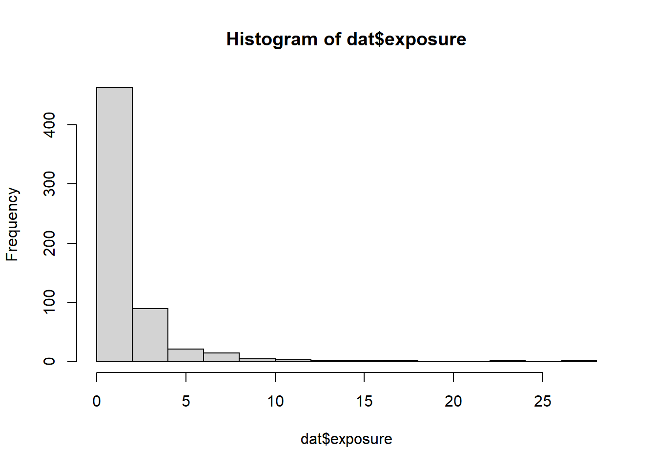
hist(dat$exposure)
hist(dat$male)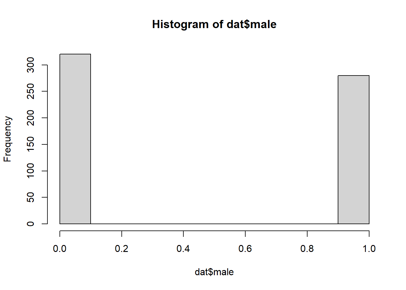 If we randomly assign individuals into treatment groups, what shape
should we expect for the within-group distributions of each
variable?
If we randomly assign individuals into treatment groups, what shape
should we expect for the within-group distributions of each
variable?
Randomization
We now create a treatment indicator by flipping a fair coin for each observation. You don’t need to know how to do this yet. Again, just run the code chunk below.
# 50/50 assignment
group <- sample(c("A","B"), size = N, replace = TRUE)
dat$group <- group

# Quick counts
table(dat$group)
##
## A B
## 280 320prop.table(table(dat$group))##
## A B
## 0.4666667 0.5333333Now create two subsets of dat.
# [Your code here]
dat_A <- dat[dat$group=="A", ]
dat_B <- dat[dat$group=="B", ]
Plot the within-subset distributions for each variable. Do they look the same? Are the two groups comparable?
# [Your code here]
hist(dat_A$IQ)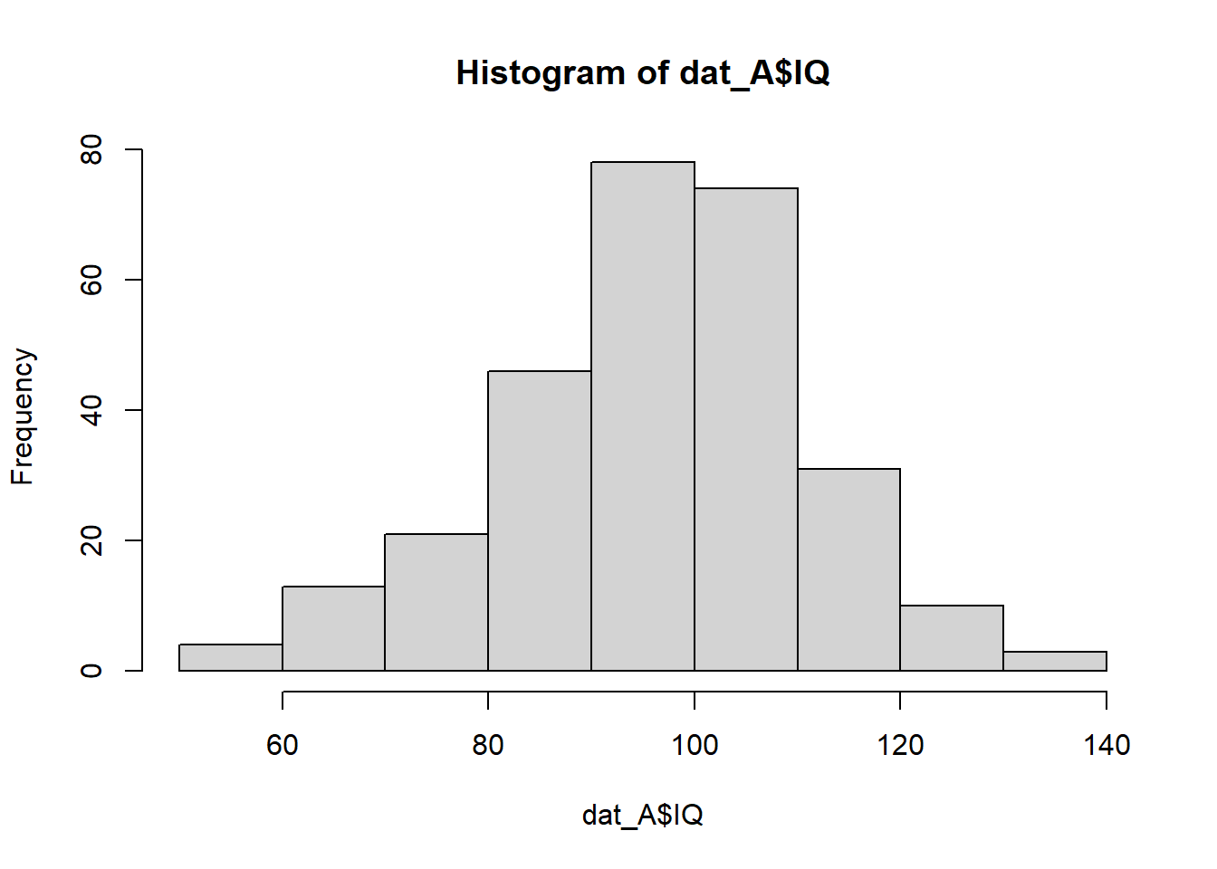
hist(dat_B$IQ)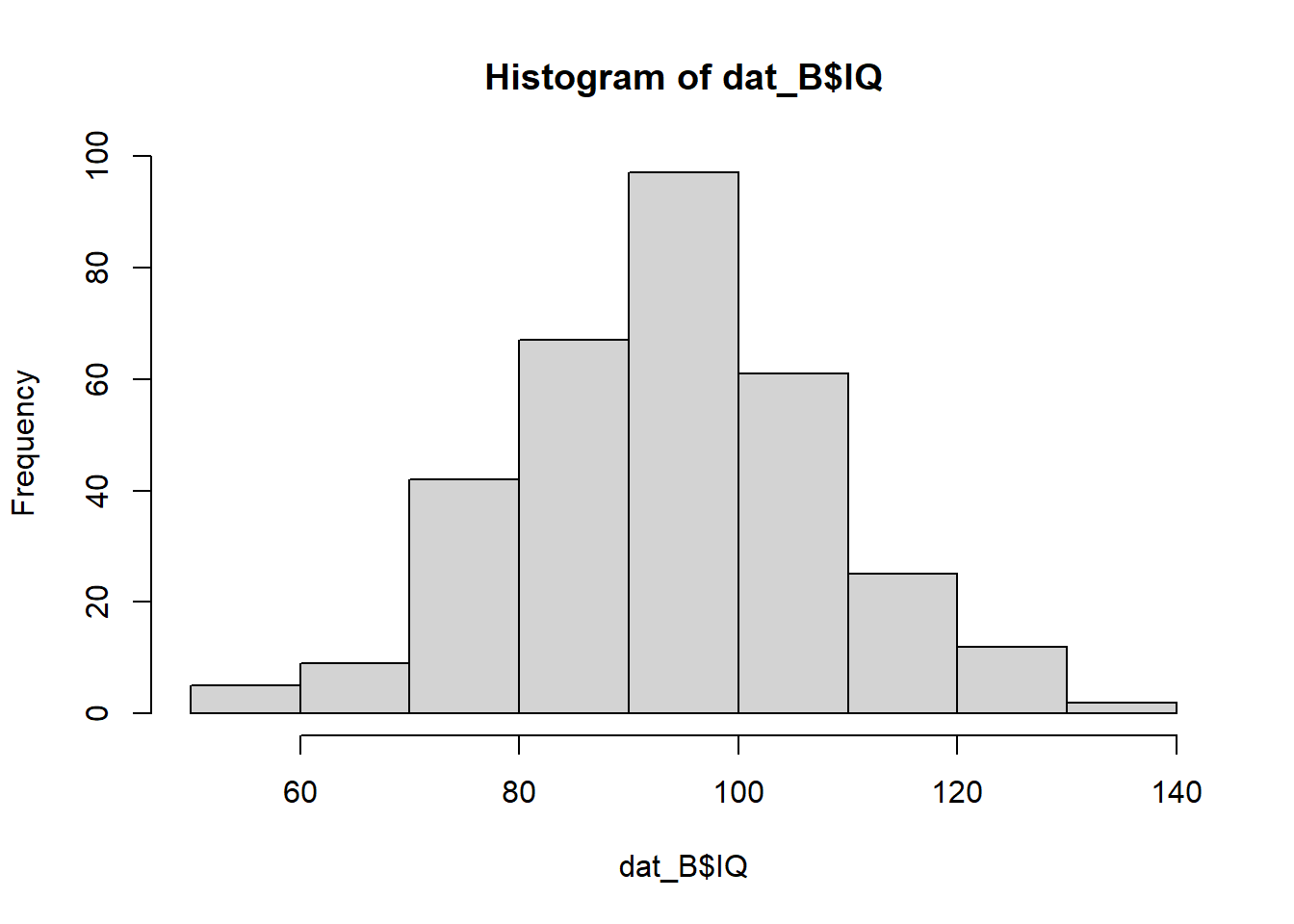
Bonus: Let’s reduce the sample size N. Are the two
groups comparable now?
Bonus: In general, how can we assess whether our two groups are comparable?
Covariate Balance
We will compute group means of each covariate using
tapply(), which we learned in class. Please calculate the
means of each variable for each subgroup. Name each as follows:
mean_groupletter_variablename.
# [Your code here]
mean_A_exposure <- tapply(dat$exposure,dat$group,mean)[["A"]]
mean_B_exposure <- tapply(dat$exposure,dat$group,mean)[["B"]]

mean_A_IQ <- tapply(dat$IQ,dat$group,mean)[["A"]]
mean_B_IQ <- tapply(dat$IQ,dat$group,mean)[["B"]]

mean_A_male <- tapply(dat$male,dat$group,mean)[["A"]]
mean_B_male <- tapply(dat$male,dat$group,mean)[["B"]]
Let’s plot the above results. You don’t need to know how to do the below yet.
balance_table <- data.frame(
  covariate = c("Exposure", "IQ", "Gender"),
  mean_A = c(mean_A_exposure, mean_A_IQ, mean_A_male),
  mean_B = c(mean_B_exposure, mean_B_IQ, mean_B_male)
)
balance_table$diff_in_means <- with(balance_table, mean_A - mean_B)
balance_table
## covariate mean_A mean_B diff_in_means
## 1 Exposure 1.8242908 1.606882 0.21740922
## 2 IQ 95.9481691 93.691826 2.25634358
## 3 Gender 0.4928571 0.443750 0.04910714For each covariate, are the A and B means close? Explain why randomization implies they should be close in expectation even if any one draw shows some noise.
Randomization as simulated counterfactuals
The potential outcomes for a unit \(i\) are \(Y_i(A)\) and \(Y_i(B)\). Randomization picks one at random to reveal. If groups are balanced on covariates and unobservables in expectation, then comparing mean outcomes between A and B estimates a causal effect.
We illustrate this by simulating an outcome Y that
depends on our covariates, but not on group
assignment.
# outcome depends on covariates (nonlinear), but not on group
Y <- 1.5 + 0.4*log(1+exposure) + 0.6*(IQ > 1.5) - 0.8*IQ + rnorm(N, 0, 0.7)
dat$Y <- Y
What is the difference in mean Y between A and B? What
would happen if assignment were correlated with one or more
covariates?
# [Your code here]