You’ll also want to reference this tutorial on ggplot.

Dataset

We’ll use the palmerpenguins dataset, which contains measurements for three penguin species (Adelie, Chinstrap, Gentoo) from the Palmer Archipelago, Antarctica. Key variables include:

species (factor: Adelie, Chinstrap, Gentoo)
island (factor)
bill_length_mm, bill_depth_mm
flipper_length_mm
body_mass_g
sex (male/female, with some missing)

We’ll focus on flipper length (in millimeters) as the outcome of interest and compare across species.

peng <- penguins
peng <- peng %>% filter(!is.na(flipper_length_mm)) # drop NAs in outcome when needed

1. What is the sample average flipper length among Gentoo penguins?

# [Your Code Here]
tapply(peng$flipper_length_mm, peng$species, mean)

##    Adelie Chinstrap    Gentoo 
##  189.9536  195.8235  217.1870

mean(peng$flipper_length_mm[peng$species == "Gentoo"])

## [1] 217.187

2. What is the sample average flipper length among Adelie penguins?

# [Your Code Here]

3. What is the estimated difference in average flipper length of Gentoo vs Adelie? Is this effect Causal?

# [Your Code Here]
mean(peng$flipper_length_mm[peng$species == "Gentoo"]) - mean(peng$flipper_length_mm[peng$species == "Adelie"]) %>%
  abs()

## [1] 27.23335

4. Visualize the distribution of `flipper_length_mm`. About how many observations are near 200 mm (±5 mm)?

Tidyverse (ggplot2) histogram

# [Your Code Here]
ggplot(data = peng, mapping = aes(x = flipper_length_mm)) +
  geom_histogram(binwidth = 10)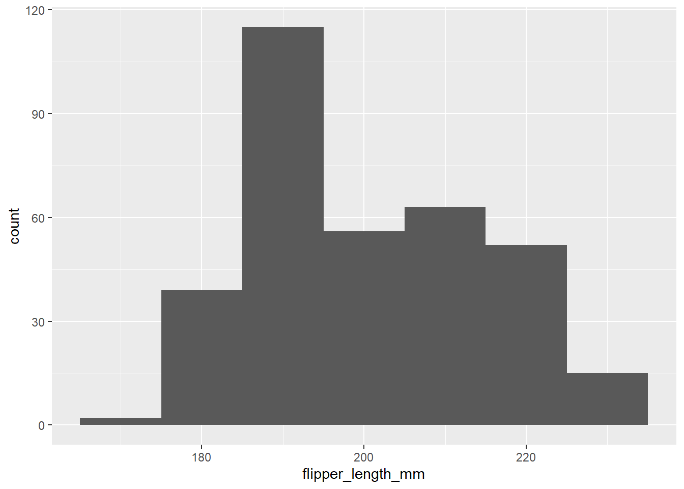

Base R histogram

# hist(peng$flipper_length_mm, breaks = seq(floor(min(peng$flipper_length_mm, na.rm = TRUE)),
#                                           ceiling(max(peng$flipper_length_mm, na.rm = TRUE)), by = 5),
#      main = "Distribution of Flipper Length (base R)",
#      xlab = "Flipper length (mm)")

Count near 200 mm

peng %>% filter(abs(flipper_length_mm -  200) < 5) %>%
  nrow()

## [1] 53

5. Explore the relationship between `flipper_length_mm` and `body_mass_g`. Does it look positive or negative?

Tidyverse (ggplot2) scatter with trend

ggplot(peng, aes(x = flipper_length_mm, y = body_mass_g)) +
  geom_point() +
  geom_smooth(method = "lm")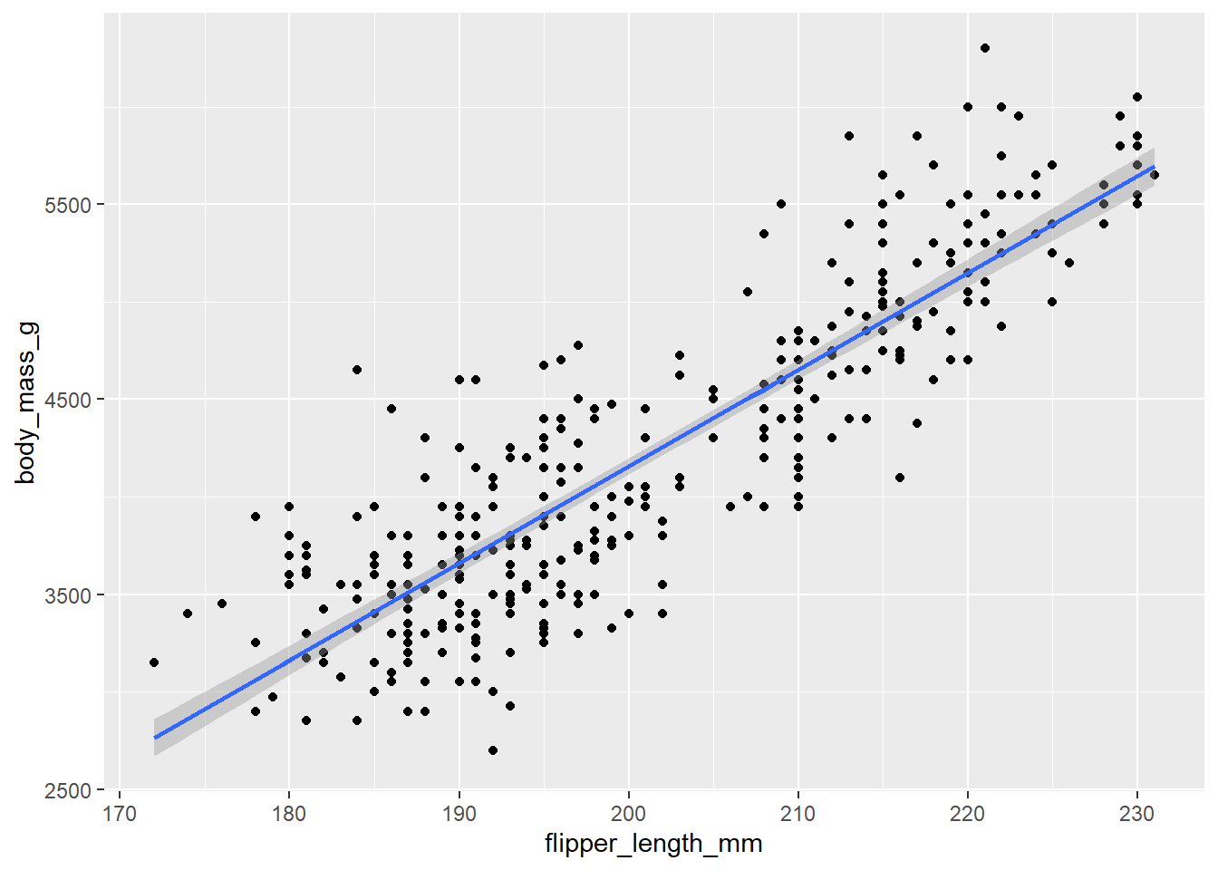

ggplot(peng, aes(y = flipper_length_mm, x = body_mass_g)) +
  geom_point() +
  geom_smooth(method = "lm")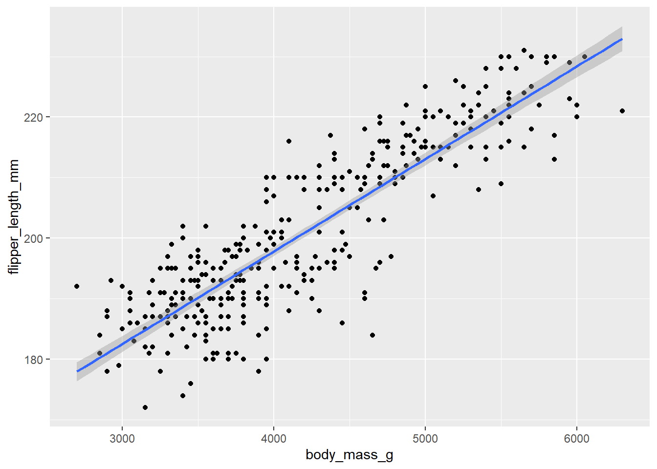

Base R scatter with fitted line

plot(peng$flipper_length_mm, peng$body_mass_g)

6. Compute the correlation between `flipper_length_mm` and `body_mass_g`.

cor(peng$flipper_length_mm, peng$body_mass_g)

## [1] 0.8712018

(a) Are you surprised by the sign? (b) Are you surprised by the absolute value (magnitude)?

7. If we wanted our estimates to generalize beyond the observed sample of penguins to all penguins of these two species, how should we select our sample?

Lab 5: Correlations and Visualizations